Two Qubit Adiabatic Sweep

Download Script · Download Job

This notebook was executed using the upstream saved emulator and hardware results. No Aquila jobs were submitted during this website build.

Job Files for Complete Examples

To be able to run the complete examples without having to submit your program to hardware and wait, you’ll need to download the associated job files. These files contain the results of running the program on the quantum hardware.

You can download the job files by clicking the “Download Job” button above. You’ll then need to place the job file in the data directory that was created for you when you ran the import part of the script (alternatively you can make the directory yourself, it should live at the same level as wherever you put this script).

Introduction

In this example, we show how to use Bloqade to program an adiabatic sweep on a pair of atoms, with the distance between atoms gradually increasing per task. This will allow us to explore the effect of the Rydberg interaction. We will run the program on both the emulator and the hardware to compare the results.

import os

import numpy as np
import matplotlib.pyplot as plt
from bloqade.analog import var, cast, load, save, start

if not os.path.isdir("data"):
    os.mkdir("data")

Defining the Program

Now, we define our program of interest. For an adiabatic protocol, we keep that Rabi frequency at a considerable value while slowly ramping the detuning from a large negative to a positive value. The idea is that when the detuning is large and negative the atoms remain in the ground state. As the detuning is ramped to positive values, the atoms are able to be excited to the Rydberg state, however if the atoms are too close together, the Rydberg interactions effectively acts like a negative detuning to neighboring atoms, preventing them from being excited. This is the blockade effect. For atoms that are sufficiently far apart, the Rydberg interaction is negligible and the atoms can be excited to the Rydberg state. As the atoms get closer together, the Rydberg interaction becomes more significant the probability of exciting both atoms becomes smaller. The typical length scale for the cross over from the non-interacting to the blockade regime is the blockade radius.

Note that you can perform arithmetic operations directly on variables in the program but this requires the variable to be explicitly declared by passing a string to the var function and THEN doing arithmetic on it.

detuning_value = var("detuning_value")
durations = cast(["ramp_time", "run_time", "ramp_time"])
prog = (
    start.add_position([(0, 0), (0, "atom_distance")])
    .rydberg.rabi.amplitude.uniform.piecewise_linear(
        durations=durations, values=[0, "rabi_value", "rabi_value", 0]
    )
    .detuning.uniform.piecewise_linear(
        durations=durations,
        values=[
            -detuning_value,
            -detuning_value,
            detuning_value,
            detuning_value,
        ],
    )
)

distances = np.arange(4, 11, 1)
batch = prog.assign(
    ramp_time=1.0, run_time=2.0, rabi_value=15.0, detuning_value=15.0
).batch_assign(atom_distance=distances)

Run on Emulator and Hardware

In previous examples, we have shown how to run a program on the emulator and hardware. First, we will run the program on the emulator and save the results to a file.

# get emulation batch, running 1000 shots per task
emu_filename = os.path.join(
    os.path.abspath(""), "data", "two-qubit-adiabatic-emulation.json"
)

if not os.path.isfile(emu_filename):
    emu_batch = batch.bloqade.python().run(1000)
    save(emu_batch, emu_filename)

Then, we can run the program on the hardware after parallelizing the tasks. We can then save the results to a file.

Hardware Execution Cost

For this particular program, 7 tasks are generated with each task having 100 shots, amounting to USD \$9.10 on AWS Braket.

filename = os.path.join(os.path.abspath(""), "data", "two-qubit-adiabatic-job.json")

if not os.path.isfile(filename):
    hardware_batch = batch.parallelize(24).braket.aquila().run_async(shots=100)
    save(hardware_batch, filename)

Plot the Results

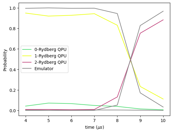
To show the blockade effect on the system, we will plot the probability of having 0, 1, or 2 Rydberg atoms as a function of time. We will do this for both the emulator and the hardware. We can use the following function to get the probabilities from the shot counts of each of the different configurations of the two Rydberg atoms: 00, 10, 01, and 11. Note that 0 corresponds to the Rydberg state while 1 corresponds to the ground state. As such, 00 corresponds to two Rydberg atoms, 10 and 01 corresponds to one Rydberg atom and one ground-state atom, and 11 corresponds to two ground-state atoms.

def rydberg_state_probabilities(emu_counts):
    probabilities_dict = {"0": [], "1": [], "2": []}

    # iterate over each of the task results
    for task_result in emu_counts:
        # get total number of shots
        total_shots = sum(task_result.values())
        # get probability of each state
        probabilities_dict["0"].append(task_result.get("11", 0) / total_shots)
        probabilities_dict["1"].append(
            (task_result.get("10", 0) + task_result.get("01", 0)) / total_shots
        )
        probabilities_dict["2"].append(task_result.get("00", 0) / total_shots)

    return probabilities_dict

Before we can plot the results we need to load the data from the files.

# get emulation report and number of shots per each state
emu_batch = load(emu_filename)

# get hardware report and number of shots per each state
hardware_batch = load(filename)
# hardware_batch.fetch()
# save(hardware_batch, filename)

We can use the rydberg_state_probabilities function to extract the probabilities from the counts. This function takes a list of counts and returns a dictionary of probabilities for each state. The counts are obtained from the report of the batch object.

Now, we can plot the results!

emu_report = emu_batch.report()
hardware_report = hardware_batch.report()

emu_rydberg_state_probabilities = rydberg_state_probabilities(emu_report.counts())
hw_rydberg_state_probabilities = rydberg_state_probabilities(hardware_report.counts())

emu_distances = emu_report.list_param("atom_distance")
hw_distances = hardware_report.list_param("atom_distance")

fig, ax = plt.subplots()
emu_colors = ["#55DE79", "#EDFF1A", "#C2477F"]  # Green, Yellow, Red

emu_lines = []
hw_lines = []
for rydberg_state, color in zip(["0", "1", "2"], emu_colors):
    (hw_line,) = ax.plot(
        emu_distances,
        hw_rydberg_state_probabilities[rydberg_state],
        label=rydberg_state + "-Rydberg QPU",
        color=color,
    )
    (emu_line,) = ax.plot(
        hw_distances,
        emu_rydberg_state_probabilities[rydberg_state],
        color="#878787",
        label="Emulator",
    )

    emu_lines.append(emu_line)
    hw_lines.append(hw_line)


ax.legend(handles=[*hw_lines, emu_lines[-1]])
ax.set_xlabel("time ($\mu s$)")
ax.set_ylabel("Probability")
fig.show()