
Quantum Scar Dynamics
Download Script · Download Job
This notebook was executed using the upstream saved emulator and hardware results. No Aquila jobs were submitted during this website build.
Introduction
In this example we show how to use Bloqade to run a quantum scar dynamics experiment. The protocol is as follows: We first prepare the atoms in a Z2 state using an adiabatic sweep. We then apply a Rabi pulse to the atoms, which will cause the atoms to oscillate but because of the Blockade effect, the atoms will not be able to transition to the Rydberg state. However, the atoms will still oscillate between the ground and some other excited many-body states.
Define the program
This notebook will also show some advanced features of Bloqade, in particular, how to
use the slice and record API to build a program that is compatible with the
hardware constraints that the rabi drive must be 0 at the end of the protocol.
The idea is that first we define the full waveform we would like to apply to the atoms
then after defining the full waveform you simply call the slice method to slice the
that waveform stopping at a variable time run_time. This works fine for detuning but
for the Rabi drive, we need to make sure that the Rabi drive is 0 at the end of the
the waveform. To do this, we use the record method to record the value of the Rabi
drive at the end of the waveform. We then use the linear method to append a segment
to the waveform that fixes the value of the Rabi drive to 0 at the end of the
waveform. Now any value of run_time will be a valid waveform that is compatible
with the hardware constraints.
import os
import numpy as npimport matplotlib.pyplot as pltfrom bloqade.analog import var, load, savefrom bloqade.analog.atom_arrangement import Chain
if not os.path.isdir("data"):    os.mkdir("data")
n_atoms = 11lattice_spacing = 6.1run_time = var("run_time")
quantum_scar_program = (    Chain(n_atoms, lattice_spacing=lattice_spacing)    # define detuning waveform    .rydberg.detuning.uniform.piecewise_linear(        [0.3, 1.6, 0.3], [-18.8, -18.8, 16.3, 16.3]    )    .piecewise_linear([0.2, 1.6], [16.3, 0.0, 0.0])    # slice the detuning waveform    .slice(start=0, stop=run_time)    # define rabi waveform    .amplitude.uniform.piecewise_linear([0.3, 1.6, 0.3], [0.0, 15.7, 15.7, 0.0])    .piecewise_linear([0.2, 1.4, 0.2], [0, 15.7, 15.7, 0])    # slice waveform, add padding for the linear segment    .slice(start=0, stop=run_time - 0.065)    # record the value of the waveform at the end of the slice to "rabi_value"    .record("rabi_value")    # append segment to waveform that fixes the value of the waveform to 0    # at the end of the waveform    .linear("rabi_value", 0, 0.065))
# get run times via the following:prep_times = np.arange(0.2, 2.2, 0.2)scar_times = np.arange(2.2, 4.01, 0.01)run_times = np.unique(np.hstack((prep_times, scar_times)))
batch = quantum_scar_program.batch_assign(run_time=run_times)
Run on Emulator and Hardware
We will run the experiment on the emulator and hardware, saving the results to disk so that we can plot them later. for more details on where these lines of code come from, see the first few tutorials.
emu_filename = os.path.join(    os.path.abspath(""), "data", "quantum-scar-dynamics-emulation.json")
if not os.path.isfile(emu_filename):    emu_batch = batch.bloqade.python().run(1000)    save(emu_batch, emu_filename)

filename = os.path.join(os.path.abspath(""), "data", "quantum-scar-dynamics-job.json")
if not os.path.isfile(filename):    hardware_batch = (        batch.parallelize(24)        .braket.aquila()        .run_async(100, ignore_submission_error=True)    )    save(hardware_batch, filename)
Plotting the results
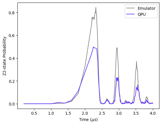
The quantity we are interested in is the probability of the atoms being in the Z2 state. We can get this by looking at the counts of the Z2 state in the report Below we define a function that will get the probability of the Z2 state for each time step in the experiment.
emu_batch = load(emu_filename)hardware_batch = load(filename)# hardware_batch.fetch()# save(hardware_batch, filename)def get_z2_probabilities(report): z2_probabilities = []
for count in report.counts(): z2_probability = count.get("01010101010", 0) / sum(list(count.values())) z2_probabilities.append(z2_probability)
return z2_probabilitiesWe can now plot the results from the emulator and hardware. We see that the emulator
emu_report = emu_batch.report()hardware_report = hardware_batch.report()
emu_run_times = emu_report.list_param("run_time")emu_z2_prob = get_z2_probabilities(emu_report)
hw_run_times = hardware_report.list_param("run_time")hw_z2_prob = get_z2_probabilities(hardware_report)
plt.plot(emu_run_times, emu_z2_prob, label="Emulator", color="#878787")plt.plot(hw_run_times, hw_z2_prob, label="QPU", color="#6437FF")
plt.legend()plt.xlabel("Time ($\mu s$)")plt.ylabel("Z2-state Probability")plt.show()