Lattice Gauge Theory Simulation

Download Script · Download Job

This notebook was executed using the upstream saved emulator and hardware results. No Aquila jobs were submitted during this website build.

Job Files for Complete Examples

To be able to run the complete examples without having to submit your program to hardware and wait, you’ll need to download the associated job files. These files contain the results of running the program on the quantum hardware.

You can download the job files by clicking the “Download Job” button above. You’ll then need to place the job file in the data directory that was created for you when you ran the import part of the script (alternatively you can make the directory yourself, it should live at the same level as wherever you put this script).

Introduction

In this notebook, we utilize Aquila to simulate the dynamics of a Lattice Gauge Theory (LGT) with a 1D Rydberg atom chain. In the realm of gauge theories, it has been discovered that the Z2 ground state and the quantum scar of the Rydberg chain correspond to the ‘string’ state and the string-inversion mechanism of the studied LGT, respectively. More intriguingly, by selectively addressing certain atoms, we can induce defects in the chain and simulate the propagation of particle-antiparticle pairs. This notebook is inspired by the paper by F. M. Surace et al. (DOI: 10.1103/PhysRevX.10.021041).

Define the Program

import os

import numpy as np
import matplotlib.pyplot as plt
from bloqade.analog import cast, load, save, piecewise_linear
from bloqade.analog.ir.location import Chain

if not os.path.isdir("data"):
    os.mkdir("data")

We introduce two new features of Bloqade here in order to accomplish this LGT simulation.

Firstly, instead of building the waveforms off the program itself using methods like .piecewise_linear and .piecewise_constant as seen in previous tutorials, we build the waveforms outside the program and then use the .apply method to put them into the program. This is similar to the Multi-qubit Blockaded Rabi Oscillations tutorial except instead of building an entire program without a geometry and then applying it on top of one, we introduce waveforms to an existing program structure.

For complex programs such as this one this makes prototyping significantly easier (you can view individual waveforms by calling .show() on them so long as there are no variables in the waveform) and keeps things modular.

Secondly, we need to be able to “selectively address” certain atoms. This is accomplished via Local Detuning where we are able to control how much of the global detuning is applied to each atom through a multiplicative scaling factor.

Bloqade has two methods of doing this (refer to the “Advanced Usage” page) but here we opt for the .scale method. We create a list of values from 0 to 1 with length equal to the number of atoms in the system. A value of 1 means the atom should experience the full detuning waveform while 0 means the atom should not experience it at all. The n-th value in the list corresponds to the n-th atom in the system.

N_atom = 13
# Setup the detuning scaling per atom.
# Note that the list of scaling values has a length equal to
# the number of atoms
detuning_ratio = [0] * N_atom
detuning_ratio[1 : (N_atom - 1) : 2] = [1, 1, 1, 1, 1, 1]
detuning_ratio[(N_atom - 1) // 2] = 1
# Notice that the detuning ratio will allow us to prepare a Z2
# ordered phase. However, the sequence of contiguous 1s in the
# middle introduce a defect.
detuning_ratio

[0, 1, 0, 1, 0, 1, 1, 1, 0, 1, 0, 1, 0]

run_time = cast("run_time")

# Define our waveforms first, then plug them into the
# program structure below
rabi_amplitude_wf = piecewise_linear(
    durations=[0.1, 2.0, 0.05, run_time, 0.05],
    values=[0, 5 * np.pi, 5 * np.pi, 4 * np.pi, 4 * np.pi, 0],
)
uniform_detuning_wf = piecewise_linear(
    durations=[2.1, 0.05, run_time + 0.05], values=[-6 * np.pi, 8 * np.pi, 0, 0]
)
local_detuning_wf = piecewise_linear(
    [0.1, 2.0, 0.05, run_time + 0.05], values=[0, -8 * 2 * np.pi, -8 * 2 * np.pi, 0, 0]
)

# Note that `scale` is called right after defining the
# global detuning
program = (
    Chain(N_atom, lattice_spacing=5.5, vertical_chain=True)
    .rydberg.rabi.amplitude.uniform.apply(rabi_amplitude_wf)
    .detuning.uniform.apply(uniform_detuning_wf)
    .scale(detuning_ratio)
    .apply(local_detuning_wf)
)

run_times = np.arange(0.0, 1.05, 0.05)
batch = program.batch_assign(run_time=run_times)

Run on Emulator and Hardware

We now run the program on both the emulator and quantum hardware.

Hardware Execution Cost

For this particular program, 21 tasks are generated with each task having 200 shots, amounting to USD \$48.30 on AWS Braket.

emu_filename = os.path.join(os.path.abspath(""), "data", "lgt-emulation.json")

if not os.path.isfile(emu_filename):
    emu_batch = batch.bloqade.python().run(1000, rtol=1e-10)
    save(emu_batch, emu_filename)

filename = os.path.join(os.path.abspath(""), "data", "lgt-job.json")

if not os.path.isfile(filename):
    hardware_batch = batch.parallelize(15).braket.aquila().run_async(shots=200)
    save(hardware_batch, filename)

Plot the Results

emu_batch = load(emu_filename)
hardware_batch = load(filename)

The following code plots the Rydberg onsite density from emulation as a function of evolution time after preparing the initial state with a defect in the middle. We observe that this defect propagates ballistically to the boundary and bounces back and forth.

emu_report = emu_batch.report()
emu_rydberg_densities = emu_report.rydberg_densities()

plt.imshow(np.array(emu_rydberg_densities).T, vmin=0, vmax=1)
plt.xticks(
    ticks=np.arange(0, 20, 2), labels=np.round(np.arange(0.0, 1.0, 0.1), 1), minor=False
)
plt.xlabel("t[us]", fontsize=14)
plt.ylabel("atom", fontsize=14)
plt.title("simulation", fontsize=14)
plt.colorbar(shrink=0.68)
plt.show()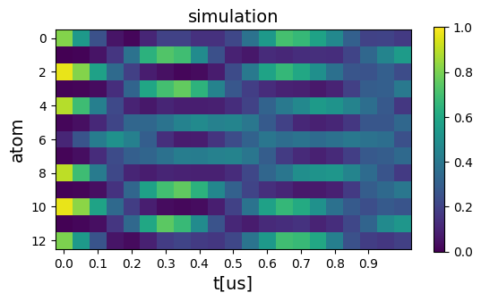

Additionally, we can plot the correlation between nearest-neighbor sites to illustrate the propagation of the defect across the chain.

def rydberg_correlation(task_bits: np.ndarray, i: int, j: int) -> np.ndarray:
    return np.mean(task_bits[:, i] * task_bits[:, j])


emu_bitstrings = emu_report.bitstrings()
bits = np.array(emu_bitstrings)
num_tasks = len(bits)
corrs = np.zeros((num_tasks, N_atom - 1), dtype=np.float64)
for task_index, task_bits in enumerate(bits):
    for i in range(N_atom - 1):
        corrs[task_index, i] = rydberg_correlation(task_bits, i, i + 1)

plt.imshow(corrs.T, vmin=0, vmax=1)
plt.xticks(
    ticks=np.arange(0, 20, 2), labels=np.round(np.arange(0.0, 1.0, 0.1), 1), minor=False
)
plt.xlabel("t[us]")
plt.ylabel("atom")
plt.title("simulation")
plt.colorbar(shrink=0.68)
plt.show()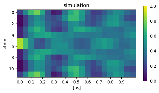

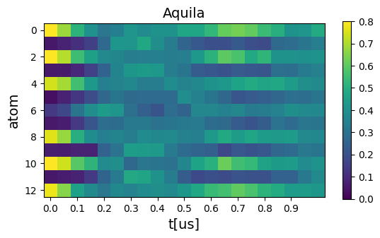
As observed below, the state with a local defect in the middle can be prepared with high fidelity on Aquila. Following the preparation stage, akin to the emulation, the defect rapidly propagates across the system.

aquila_rydberg_densities = hardware_batch.report().rydberg_densities()

plt.imshow(np.array(aquila_rydberg_densities).T, vmin=0, vmax=0.8)
plt.xticks(
    ticks=np.arange(0, 20, 2), labels=np.round(np.arange(0.0, 1.0, 0.1), 1), minor=False
)
plt.xlabel("t[us]", fontsize=14)
plt.ylabel("atom", fontsize=14)
plt.title("Aquila", fontsize=14)
plt.colorbar(shrink=0.68)
plt.show()