
Single Qubit Floquet Dynamics
Download Script · Download Job
This notebook was executed using the upstream saved emulator and hardware results. No Aquila jobs were submitted during this website build.
Introduction
Rounding out the single qubit examples we will show how to generate a Floquet protocol. We will define the protocol using a python function and then use the Bloqade API to sample the function at certain intervals to make it compatible with the hardware, which only supports piecewise linear/constant functions. First let us start with the imports.
import os
import numpy as npimport matplotlib.pyplot as pltfrom bloqade.analog import cast, load, save, start
if not os.path.isdir("data"):    os.mkdir("data")
Define the program.
For the Floquet protocol we keep We do the same Rabi drive but allow the detuning to
vary sinusoidally. We do this by defining a smooth function for the detuning and then
sampling it at certain intervals (in this case, the minimum hardware-supported time
step). Note that the sample method will always sample at equal to or greater than
the specified time step. If the total time interval is not divisible by the time
step, the last time step will be larger than the specified time step. Also note that
the arguments of your function must be named arguments, e.g. no *args or **kwargs,
because Bloqade will analyze the function signature to and generate variables for
each argument.
min_time_step = 0.05
durations = cast(["ramp_time", "run_time", "ramp_time"])

def detuning_wf(t, drive_amplitude, drive_frequency):    return drive_amplitude * np.sin(drive_frequency * t)

floquet_program = (    start.add_position((0, 0))    .rydberg.rabi.amplitude.uniform.piecewise_linear(        durations, [0, "rabi_max", "rabi_max", 0]    )    .detuning.uniform.fn(detuning_wf, sum(durations))    .sample("min_time_step", "linear"))
We assign values to the necessary variables and then run_async the program to both the emulator and actual hardware.
run_times = np.linspace(0.05, 3.0, 101)
floquet_job = floquet_program.assign(    ramp_time=0.06,    min_time_step=0.05,    rabi_max=15,    drive_amplitude=15,    drive_frequency=15,).batch_assign(run_time=run_times)
have to start the time at 0.05 because the hardware does not support anything less than that time step. We can now run_async the job to the emulator and hardware.
Run Emulator and Hardware
Like in the first tutorial, we will run the program on the emulator and hardware.
Note that for the hardware we will use the parallelize method to run multiple
copies of the program in parallel. For more information about this process, see the
first tutorial.
emu_filename = os.path.join(os.path.abspath(""), "data", "floquet-emulation.json")print(emu_filename)
if not os.path.isfile(emu_filename):    emu_batch = floquet_job.bloqade.python().run(10000)    save(emu_batch, emu_filename)
hardware_filename = os.path.join(os.path.abspath(""), "data", "floquet-job.json")
if not os.path.isfile(hardware_filename): batch = floquet_job.parallelize(24).braket.aquila().run_async(shots=50) save(batch, hardware_filename)/tmp/analog-floquet-dynamics-bxlcnka1/data/floquet-emulation.jsonPlotting the Results
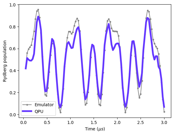
Exactly like in the Rabi Oscillation example, we can now plot the results from the
hardware and emulation together. Again we will use the report to calculate the mean
Rydberg population for each run, and then plot the results.
first we load the results from the emulation and hardware.
emu_batch = load(emu_filename)assert not isinstance(emu_batch, dict)hardware_batch = load(hardware_filename)assert not isinstance(hardware_batch, dict)# hardware_batch.fetch()# save(filename, hardware_batch)Next we extract the run times and the Rydberg population from the report. We can then plot the results.
hardware_report = hardware_batch.report()emulator_report = emu_batch.report()
times = emulator_report.list_param("run_time")density = [1 - ele.mean() for ele in emulator_report.bitstrings()]plt.plot(times, density, color="#878787", marker=".", label="Emulator")
times = hardware_report.list_param("run_time")density = [1 - ele.mean() for ele in hardware_report.bitstrings()]
plt.plot(times, density, color="#6437FF", linewidth=4, label="QPU")plt.xlabel("Time ($\mu s$)")plt.ylabel("Rydberg population")plt.legend()plt.show()