
1D Z2 State Preparation
Download Script · Download Job
This notebook was executed using the upstream saved emulator and hardware results. No Aquila jobs were submitted during this website build.
Introduction
In this example we show how to create the Z2 ordered phase on a 1D chain of atoms and how to perform a scan over the sweep time to understand the behavior of an adiabatic sweep and the effect of the Rydberg blockade on a many-body system.
Let’s import all the tools we’ll need.
import os
import numpy as npimport matplotlib.pyplot as pltfrom bloqade.analog import load, savefrom bloqade.analog.atom_arrangement import Chain
if not os.path.isdir("data"):    os.mkdir("data")
Program Definition
We define a program where our geometry is a chain of 11 atoms with a distance of 6.1 micrometers between atoms.
The pulse schedule presented here should be reminiscent of the Two Qubit Adiabatic Sweep example although we’ve opted to reserve variable usage for values that will actually have their parameters swept.
# Define relevant parameters for the lattice geometry and pulse schedulen_atoms = 11lattice_spacing = 6.1min_time_step = 0.05We choose a maximum Rabi amplitude of 15.8 MHz. Pushing the Rabi amplitude as high as we can minimizes the protocol duration, but maintains the same pulse area, . For this reason, in many cases, maximizing the Rabi frequency is considered good practice for minimizing decoherence effects.
rabi_amplitude_values = [0.0, 15.8, 15.8, 0.0]The lattice spacing and Rabi amplitudes give us a nearest neighbor interaction strength: where is our van der Waals coefficient for Aquila hardware and is the lattice spacing we defined earlier. Our interaction strength for next-nearest neighbors is quite low comparatively: The Rydberg interaction term dominates for nearest neighbor spacing, while the Rabi coupling dominates for next-nearest neighbors. This increases the probability of realizing a Rydberg blockade for nearest neighbors, but decreases the probability of Rydberg interaction between next-nearest neighbors. So far, we’re in a good position for creating a Z2 phase.
Next, we define our detuning values.
rabi_detuning_values = [-16.33, -16.33, 16.33, 16.33]We start at large negative detuning values where all atoms are in the ground state. Then, we transition to large positive detuning values where the Rydberg state becomes energetically favorable and inter-atomic interactions become more important.
The maximum absolute detuning value of gives us a Rydberg blockade radius Typically, we define the lattice spacing such that for a good blockade approximation and Z2 state probability.
Lastly, we define a set of test durations over which to execute our pulses and write the instructions for our program.
durations = [0.8, "sweep_time", 0.8]# Note the addition of a "sweep_time" variable# for performing sweeps of time values.
time_sweep_z2_prog = (    Chain(n_atoms, lattice_spacing=lattice_spacing)    .rydberg.rabi.amplitude.uniform.piecewise_linear(durations, rabi_amplitude_values)    .detuning.uniform.piecewise_linear(durations, rabi_detuning_values))
# Allow "sweep_time" to assume values from 0.05 to 2.4 microseconds for a total of# 20 possible values.# Starting at exactly 0.0 isn't feasible so we use the `min_time_step` defined# previously.time_sweep_z2_job = time_sweep_z2_prog.batch_assign(    sweep_time=np.linspace(min_time_step, 2.4, 20))
Running on the Emulator and Hardware
With our program properly composed we can now easily send it off to both the emulator and hardware.
We select the Braket emulator and tell it that for each variation of the “time_sweep” variable we’d like to run 10000 shots. For the hardware we take advantage of the fact that 11 atoms takes up so little space on the machine we can duplicate that geometry multiple times to get more data per shot. We set a distance of 24 micrometers between copies to minimize potential interactions between them.
For both cases, to allow us to submit our program without having to wait on immediate results from hardware (which could take a while considering queueing and window restrictions), we save the necessary metadata to a file that can then be reloaded later and results fetched when they are available.
emu_filename = os.path.join(os.path.abspath(""), "data", "time-sweep-emulation.json")if not os.path.isfile(emu_filename):    emu_future = time_sweep_z2_job.bloqade.python().run(shots=10000)    save(emu_future, emu_filename)
filename = os.path.join(os.path.abspath(""), "data", "time-sweep-job.json")if not os.path.isfile(filename):    future = time_sweep_z2_job.parallelize(24).braket.aquila().run_async(shots=100)    save(future, filename)
Plotting the Results
To make our lives easier we define a trivial function to
extract the probability of the Z2 phase from each of the tasks generated from the
parameter sweep. The counts are obtained from the reportof the batch object.
def get_z2_probabilities(report):    z2_probabilities = []
    for count in report.counts():        z2_probability = count["01010101010"] / sum(list(count.values()))        z2_probabilities.append(z2_probability)
    return z2_probabilities
Extracting Counts And Probabilities
We will now extract the counts and probabilities from the emulator and hardware runs. We will then plot the results. First we load the data from the files:
# retrieve results from HWemu_batch = load(emu_filename)hardware_batch = load(filename)
# Uncomment lines below to fetch results from Braket# hardware_batch = hardware_batch.fetch()# save(hardware_batch, filename)
To get the counts we need to get a report from the batch objects. Then with the report we can get the counts. The counts are a dictionary that maps the bitstring to the number of times that bitstring was measured.
emu_report = emu_batch.report()hardware_report = hardware_batch.report()emu_probabilities = get_z2_probabilities(emu_report)hardware_probabilities = get_z2_probabilities(hardware_report)
emu_sweep_times = emu_report.list_param("sweep_time")hardware_sweep_times = hardware_report.list_param("sweep_time")

plt.plot(emu_sweep_times, emu_probabilities, label="Emulator", color="#878787")plt.plot(hardware_sweep_times, hardware_probabilities, label="QPU", color="#6437FF")
plt.legend()plt.show()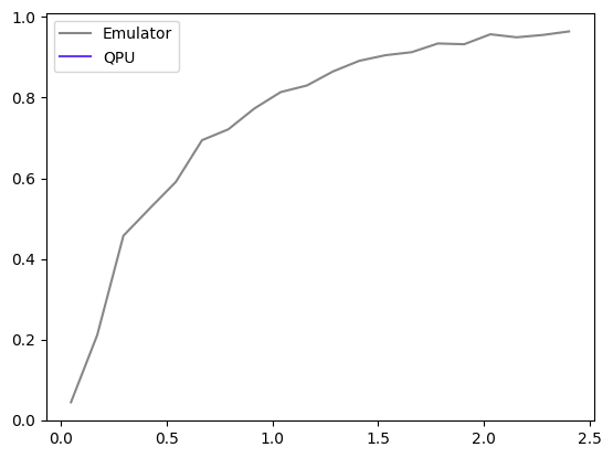
We can also plot the emulated Z2 ordered phase for a specific sweep time. Here, we extract data for a sweep time of or a total pulse duration of .
densities = emu_report.rydberg_densities()site_indices = densities.loc[0].index.valuesrydberg_densities_67_sweep = densities.loc[5, 0:10].values
plt.bar(site_indices, rydberg_densities_67_sweep, color="#C8447C")plt.xticks(site_indices)plt.title("Z2 Phase Rydberg Densities for 2.27$\mu$s Total Pulse Duration")plt.xlabel("Atom Site Index")plt.ylabel("Rydberg Density")
plt.show()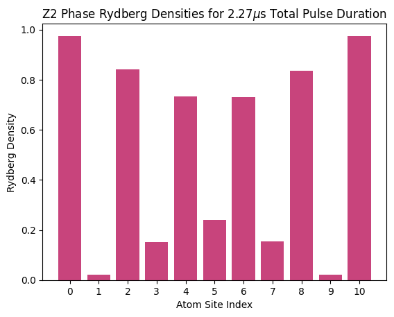
Similarly, we can visualize the emulated Rydberg densities of each site index as the sweep time increases and we approach adiabatic evolution.
rydberg_densities = densities.values.transpose()
im = plt.imshow(rydberg_densities)plt.xticks(rotation=90)plt.xticks(    [x for x in range(len(emu_sweep_times))], [round(dur, 2) for dur in emu_sweep_times])plt.yticks(site_indices)plt.xlabel("Sweep Time ($\mu$s)")plt.ylabel("Atom Site Index")plt.colorbar(im, shrink=0.6)
plt.show()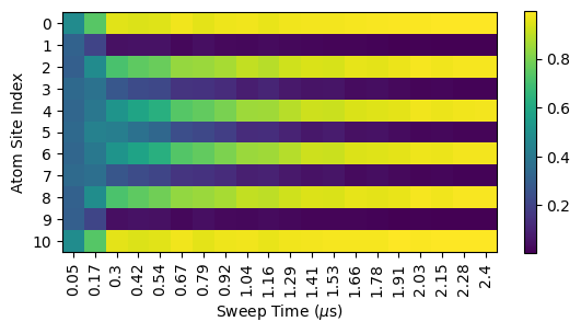
Analysis
As expected, we see that if we allow the pulse schedule to run for a longer and longer period of time (more “adiabatically”) we have an increasing probability of creating the Z2 phase.