
Multi-qubit Blockaded Rabi Oscillations
Download Script · Download Job
This notebook was executed using the upstream saved emulator and hardware results. No Aquila jobs were submitted during this website build.
Introduction
In this tutorial we will show you how to compose geometries with pulse sequences to perform multi-qubit blockaded Rabi oscillations. The Physics here is described in detail in the whitepaper. But in short, we can use the Rydberg blockade to change the effective Rabi frequency of the entire system by adding more atoms to the cluster.
import os
import numpy as npimport matplotlib.pyplot as pltfrom bloqade.analog import load, save, startfrom bloqade.analog.atom_arrangement import Chain, Square
if not os.path.isdir("data"):    os.mkdir("data")
Defining the Geometry
We will start by defining the geometry of the atoms. The idea here is to cluster
the atoms so that they are all blockaded from each other. Using a combination of the
Chain and Square classes, as a base, one can add additional atoms to the geometry
using the add_position method. This method takes a list of tuples, or a single
tuple, of the form (x,y) where x and y are the coordinates of the atom in units
of the lattice constant.
distance = 4.0inv_sqrt_2_rounded = 2.6
geometries = {    1: Chain(1),    2: Chain(2, lattice_spacing=distance),    3: start.add_position(        [(-inv_sqrt_2_rounded, 0.0), (inv_sqrt_2_rounded, 0.0), (0, distance)]    ),    4: Square(2, lattice_spacing=distance),    7: start.add_position(        [            (0, 0),            (distance, 0),            (-0.5 * distance, distance),            (0.5 * distance, distance),            (1.5 * distance, distance),            (0, 2 * distance),            (distance, 2 * distance),        ]    ),}
Defining the Pulse Sequence
Next, we will define the pulse sequence. We start from the start object, which is
an empty list of atom locations. In this case, we do not need atoms to build the pulse
sequence, but to extract the sequence, we need to call the parse_sequence method.
This creates a Sequence object that we can apply to multiple geometries.
sequence = start.rydberg.rabi.amplitude.uniform.piecewise_linear( durations=["ramp_time", "run_time", "ramp_time"], values=[0.0, "rabi_drive", "rabi_drive", 0.0],).parse_sequence()Defining the Program
Now, all that is left to do is to compose the geometry and the Pulse sequence into a
fully defined program. We can do this by calling the apply method on the geometry
and passing in the sequence. This method will return an object that can then be
assigned parameters.
batch = ( geometries[7] .apply(sequence) .assign(ramp_time=0.06, rabi_drive=5) .batch_assign(run_time=0.05 * np.arange(21)))Run Emulator and Hardware
Again, we run the program on the emulator and Aquila and save the results to a file so we can use them later.
emu_filename = os.path.join(    os.path.abspath(""), "data", "multi-qubit-blockaded-emulation.json")
if not os.path.isfile(emu_filename):    emu_batch = batch.bloqade.python().run(10000, interaction_picture=True)    save(emu_batch, emu_filename)
filename = os.path.join(os.path.abspath(""), "data", "multi-qubit-blockaded-job.json")
if not os.path.isfile(filename):    hardware_batch = batch.parallelize(24).braket.aquila().run_async(shots=100)    save(hardware_batch, filename)
Plotting the Results
First, we load the results from the file.
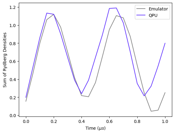
emu_batch = load(emu_filename)hardware_batch = load(filename)# hardware_batch.fetch()# save(filename, hardware_batch)The quantity of interest here is the total Rydberg density of the cluster defined as
the sum of the Rydberg densities of each atom. We can extract this from the results
and plot it as a function of time. We will do this for both the emulator and the
hardware. We can use the rydberg_densities function to extract the densities from
the Report of the batch object.
emu_report = emu_batch.report()emu_densities = emu_report.rydberg_densities()emu_densities_summed = emu_densities.sum(axis=1)
hardware_report = hardware_batch.report()hardware_densities = hardware_report.rydberg_densities()hardware_densities_summed = hardware_densities.sum(axis=1)

emu_run_times = emu_report.list_param("run_time")hw_run_times = hardware_report.list_param("run_time")
fig, ax = plt.subplots()ax.set_xlabel("Time")ax.set_ylabel("Sum of Rydberg Densities")# emulationax.plot(emu_run_times, emu_densities_summed, label="Emulator", color="#878787")# hardwareax.plot(hw_run_times, hardware_densities_summed, label="QPU", color="#6437FF")ax.legend()ax.set_xlabel("Time ($\mu s$)")ax.set_ylabel("Sum of Rydberg Densities")plt.show()