
Nonequilibrium Dynamics of nearly Blockaded Rydberg Atoms
Download Script · Download Job
This notebook was executed using the upstream saved emulator and hardware results. No Aquila jobs were submitted during this website build.
Introduction
In this example we will show how to generate multi-atom programs looking specifically at the dynamics of two atoms that are right on the blockade radius. First let’s start with the imports.
import os
import numpy as npimport matplotlib.pyplot as pltfrom bloqade.analog import load, savefrom bloqade.analog.atom_arrangement import Chain
if not os.path.isdir("data"):    os.mkdir("data")
Program Definition
We will start by defining a program. We set up a chain of two atoms
with a parameterized distance between them. We then define a Rabi
like in the original Rabi oscillation example. Given a rabi_ampl of 15 rad/µs
the blockaded radius s 8.44 µm. We will look at the dynamics of the system for a
distance of 8.5 µm to be every so slightly outside of the blockade radius. We then
define a batch of programs for different run_time values.
initial_geometry = Chain(2, lattice_spacing="distance")program_waveforms = initial_geometry.rydberg.rabi.amplitude.uniform.piecewise_linear( durations=["ramp_time", "run_time", "ramp_time"], values=[0.0, "rabi_ampl", "rabi_ampl", 0.0],)program_assigned_vars = program_waveforms.assign( ramp_time=0.06, rabi_ampl=15, distance=8.5)batch = program_assigned_vars.batch_assign(run_time=0.05 * np.arange(31))Run Emulator and Hardware
Once again we will run the emulator and hardware. We will use the
local_emulator method to run the emulator locally. We will then
save the results to a file so that we can use them later.
emu_filename = os.path.join( os.path.abspath(""), "data", "nonequilibrium-dynamics-blockade-emulation.json")if not os.path.isfile(emu_filename): emu_batch = batch.bloqade.python().run(10000) save(emu_batch, emu_filename)When running on the hardware we will also parallelize the batch and submit.
filename = os.path.join(    os.path.abspath(""), "data", "nonequilibrium-dynamics-blockade-job.json")
if not os.path.isfile(filename):    hardware_batch = batch.parallelize(24).braket.aquila().run_async(shots=100)    save(hardware_batch, filename)
Plotting the Results
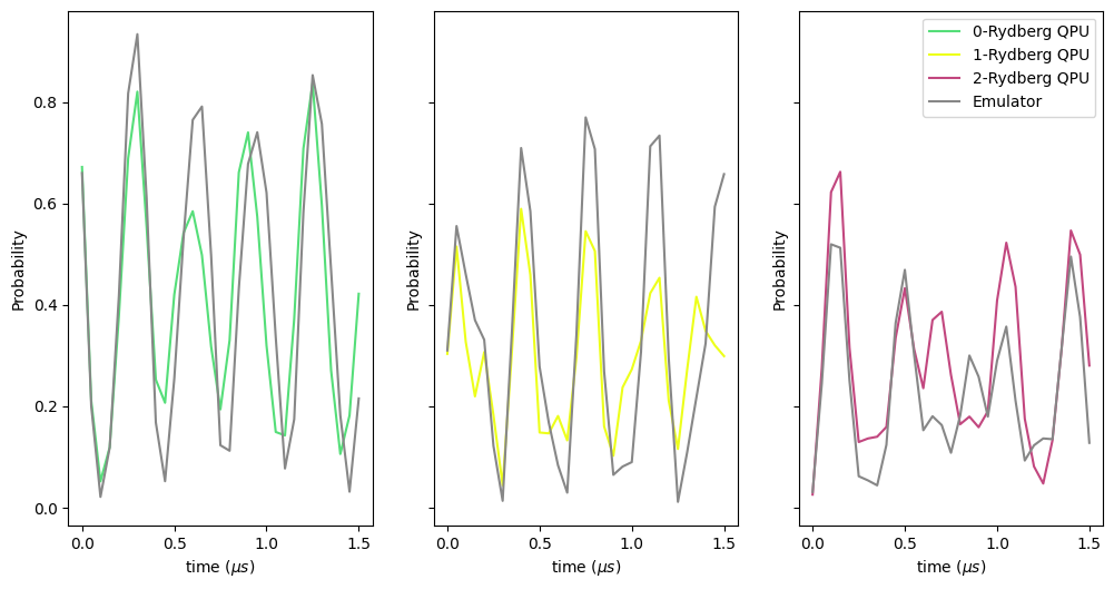
In order to show the complex dynamics we will plot the probability of having 0, 1
, or 2 Rydberg atoms as a function of time. We will do this for both the emulator
and the hardware. We can use the rydberg_state_probabilities function to extract
the probabilities from the counts. This function takes a list of counts and returns a
dictionary of probabilities for each state. The counts are obtained from the report
of the batch object.
def rydberg_state_probabilities(shot_counts):    probabilities_dict = {"0": [], "1": [], "2": []}
    # iterate over each of the task results    for task_result in shot_counts:        # get total number of shots        total_shots = sum(task_result.values())        # get probability of each state        probabilities_dict["0"].append(task_result.get("11", 0) / total_shots)        probabilities_dict["1"].append(            (task_result.get("10", 0) + task_result.get("01", 0)) / total_shots        )        probabilities_dict["2"].append(task_result.get("00", 0) / total_shots)
    return probabilities_dict
Extracting the counts and probabilities
We will now extract the counts and probabilities from the emulator and hardware runs. We will then plot the results. First we load the data from the files.
emu_batch = load(emu_filename)emu_report = emu_batch.report()emu_counts = emu_report.counts()
hardware_batch = load(filename)# hardware_batch.fetch() # uncomment to fetch results from Braket# save(filename, hardware_batch)
To get the counts we need to get a report from the batch objects. Then with the
report we can get the counts. The counts are a dictionary that maps the bitstring to
the number of times that bitstring was measured.
emu_report = emu_batch.report()hardware_report = hardware_batch.report()

emu_rydberg_state_probabilities = rydberg_state_probabilities(emu_report.counts())hw_rydberg_state_probabilities = rydberg_state_probabilities(hardware_report.counts())
plot 0, 1, and 2 Rydberg state probabilities but in separate plots
figure, axs = plt.subplots(1, 3, figsize=(12, 6), sharey=True)
emu_run_times = emu_report.list_param("run_time")hardware_run_times = hardware_report.list_param("run_time")
emu_colors = ["#55DE79", "#EDFF1A", "#C2477F"]  # Green, Yellow, Red
emu_lines = []hw_lines = []for ax, rydberg_state, color in zip(axs, ["0", "1", "2"], emu_colors):    (hw_line,) = ax.plot(        emu_run_times,        hw_rydberg_state_probabilities[rydberg_state],        label=rydberg_state + "-Rydberg QPU",        color=color,    )    (emu_line,) = ax.plot(        hardware_run_times,        emu_rydberg_state_probabilities[rydberg_state],        color="#878787",    )    emu_line.set_label("Emulator")
    emu_lines.append(emu_line)    hw_lines.append(hw_line)
    ax.set_xlabel("time ($\mu s$)")    ax.set_ylabel("Probability")
ax.legend(handles=[*hw_lines, emu_lines[-1]])
plt.show()