Single Qubit Rabi Oscillations

Download Script · Download Job

This notebook was executed using the upstream saved emulator and hardware results. No Aquila jobs were submitted during this website build.

Job Files for Complete Examples

To be able to run the complete examples without having to submit your program to hardware and wait, you’ll need to download the associated job files. These files contain the results of running the program on the quantum hardware.

You can download the job files by clicking the “Download Job” button above. You’ll then need to place the job file in the data directory that was created for you when you ran the import part of the script (alternatively you can make the directory yourself, it should live at the same level as wherever you put this script).

Introduction

In this example we show how to use Bloqade to emulate Rabi oscillations of a Neutral Atom and run it on hardware. We will define a Rabi oscillation as a sequence with a constant detuning and Rabi frequency. In practice, the Rabi frequency has to start and end at 0.0, so we will use a piecewise linear function to ramp up and down the Rabi frequency.

import os

import numpy as np
import matplotlib.pyplot as plt
from bloqade.analog import cast, load, save, start

if not os.path.isdir("data"):
    os.mkdir("data")

Define the program.

Below we define program with one atom, with constant detuning but variable Rabi frequency, ramping up to “rabi_ampl” and then returning to 0.0. Note that the cast function can be used to create a variable that can used in multiple places in the program. These variables support basic arithmetic operations, such as addition, subtraction, multiplication, and division. They also have min and max methods that can be used in place of built-in python min and max functions, e.g. cast("a").min(cast("b")).

durations = cast(["ramp_time", "run_time", "ramp_time"])

rabi_oscillations_program = (
    start.add_position((0, 0))
    .rydberg.rabi.amplitude.uniform.piecewise_linear(
        durations=durations, values=[0, "rabi_ampl", "rabi_ampl", 0]
    )
    .detuning.uniform.constant(duration=sum(durations), value="detuning_value")
)

Assign values to the variables in the program,

Once your program is built, you can use the assign method to assign values to the variables in the program. These values must be numeric, and can be either int, float, or Decimal (from the decimal module). Note that the Decimal type is used to represent real numbers exactly, whereas float is a 64-bit floating point number that is only accurate to about 15 decimal places. The Decimal type is recommended for Bloqade programs, as it will ensure that your program is simulated and run with the highest possible precision. We can also do a parameter scan using the batch_assign method, which will create a different program for each value provided in the list. In this case, we are sweeping the run_time variable, which is the time that the Rabi amplitude stays at the value of rabi_ampl.

run_times = np.linspace(0, 3, 101)

rabi_oscillation_job = rabi_oscillations_program.assign(
    ramp_time=0.06, rabi_ampl=15, detuning_value=0.0
).batch_assign(run_time=run_times)

Run Emulator and Hardware

To run the program on the emulator we can select the bloqade provider as a property of the batch object. Bloqade has its own emulator that we can use to run the program. To do this select python() as the next option followed by the run method. Then we dump the results to a file so that we can use them later. Note that unlike the actual hardware the shots do not correspond to multiple executions of the emulator, but rather the number of times the final wavefunction is sampled. This is because the emulator does not simulate any noise.

emu_filename = os.path.join(os.path.abspath(""), "data", "rabi-emulation.json")

if not os.path.isfile(emu_filename):
    emu_batch = rabi_oscillation_job.bloqade.python().run(10000)
    save(emu_batch, emu_filename)

When running on the hardware we can use the braket provider. However, we will need to specify the device to run on. In this case we will use Aquila via the aquila method. Before that we must note that because Aquila can support up to 256 atoms in an area that is $75 \times 76 \mu m^2$. We need to make full use of the capabilities of the device. Bloqade automatically takes care of this with the parallelize method, which will allow us to run multiple copies of the program in parallel using the full user provided area of Aquila. The parallelize method takes a single argument, which is the distance between each copy of the program on a grid. In this case, we want to make sure that the distance between each atom is at least 24 micrometers, so that the Rydberg interactions between atoms are negligible.

To run the program but not wait for the results, we can use the run_async method, which will return a Batch object that can be used to fetch the results later. After running the program, we dump the results to a file so that we can use them later. Note that if you want to wait for the results in the python script just call the run method instead of run_async. This will block the script until all results in the batch are complete.

Hardware Execution Cost

For this particular program, 101 tasks are generated with each task having 1000 shots, amounting to USD \$1040.30 on AWS Braket.

hardware_filename = os.path.join(os.path.abspath(""), "data", "rabi-job.json")

if not os.path.isfile(hardware_filename):
    batch = rabi_oscillation_job.parallelize(24).braket.aquila().run_async(1000)
    save(batch, hardware_filename)

Plotting the Results

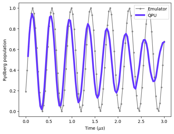
The quantity of interest in this example is the probability of finding the atom in the Rydberg state, which is given by the 0 measurement outcome. The reason that 0 is the Rydberg state is because the in the actual device the Rydberg atoms are pushed out of the trap area and show up as a dark spot in the image. To get the probability of being in the Rydberg state, we can use the bitstrings method of the Report object, which returns a list of numpy arrays containing the measurement outcomes for each shot. We can then use the mean method of the numpy array to get the probability of being in the Rydberg state for each shot. We can then plot the results as a function of time. the time value can be obtained from the run_time parameter of the Report object as a list.

before that we need to load the results from our previously saved files using the load function from bloqade.analog:

emu_batch = load(emu_filename)
hardware_batch = load(hardware_filename)
# hardware_batch.fetch()
# save(filename, hardware_batch)

hardware_report = hardware_batch.report()
emulator_report = emu_batch.report()

times = emulator_report.list_param("run_time")
density = [1 - ele.mean() for ele in emulator_report.bitstrings()]
plt.plot(times, density, color="#878787", marker=".", label="Emulator")

times = hardware_report.list_param("run_time")
density = [1 - ele.mean() for ele in hardware_report.bitstrings()]
plt.plot(times, density, color="#6437FF", linewidth=4, label="QPU")

plt.xlabel("Time ($\mu s$)")
plt.ylabel("Rydberg population")
plt.legend()
plt.show()