
Overview
Tsim is a quantum circuit sampler that can efficiently sample from Clifford+T circuits with Pauli noise. It is based on ZX-calculus stabilizer rank decomposition and parametrized ZX diagrams, following work of arXiv:2403.06777.
Supported Gates
Tsim supports a universal gate set, together with measurement and reset instructions, and Pauli noise channels.
Clifford Instructions
Tsim supports all instructions supported by Stim. Below, we show the standard generating set of Clifford gates:
from tsim import Circuit
c = Circuit("H 0")print(c.to_matrix())c.diagram("timeline-svg", height=120)
[[ 0.70710678+0.j 0.70710678+0.j] [ 0.70710678+0.j -0.70710678+0.j]]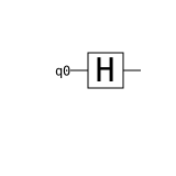
c = Circuit("S 0")print(c.to_matrix())c.diagram("timeline-svg", height=120)[[ 1.+0.j 0.-0.j] [-0.+0.j 0.+1.j]]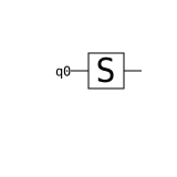
c = Circuit("CNOT 0 1")print(c.to_matrix())c.diagram("timeline-svg", height=160)[[ 1.+0.j 0.+0.j -0.+0.j 0.+0.j] [ 0.+0.j 1.+0.j 0.+0.j -0.+0.j] [ 0.+0.j -0.+0.j 0.+0.j 1.+0.j] [-0.+0.j 0.+0.j 1.+0.j 0.+0.j]]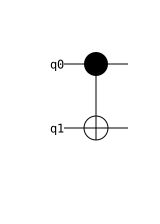
Non-Clifford Instructions
In addition to Clifford gates, Tsim supports the following non-Clifford gates. Note that all rotation parameters are defined in units of .
Computation time and memory requirement scales exponentially with the number of non-Clifford gates.
c = Circuit("T 0")print(c.to_matrix())c.diagram("timeline-svg", height=120)[[ 1. +0.j 0. +0.j ] [-0. +0.j 0.70710678+0.70710678j]]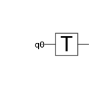
c = Circuit("R_X(0.1) 0") # rotation around X-axis by 0.1πprint(c.to_matrix())c.diagram("timeline-svg", height=120)[[ 0.98768834-0.j 0. -0.15643447j] [-0. -0.15643447j 0.98768834-0.j ]]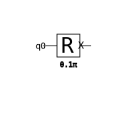
c = Circuit("R_Y(0.1) 0") # rotation around Y-axis by 0.1πprint(c.to_matrix())c.diagram("timeline-svg", height=120)[[ 0.98768834-0.j -0.15643447+0.j] [ 0.15643447-0.j 0.98768834-0.j]]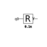
c = Circuit("R_Z(0.1) 0") # rotation around Z-axis by 0.1πprint(c.to_matrix())c.diagram("timeline-svg", height=120)[[ 0.98768834-0.15643447j 0. +0.j ] [-0. +0.j 0.98768834+0.15643447j]]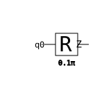
c = Circuit("U3(0.1, 0.2, 0.3) 0")print(c.to_matrix())c.diagram("timeline-svg", height=120)[[ 0.98768834-0.j -0.09194987-0.12655814j] [ 0.12655814+0.09194987j 0. +0.98768834j]]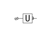
Measurement and Reset instructions
Tsim supports all collapsing gates supported by Stim.
c = Circuit("M 0")c.diagram("timeline-svg", height=120)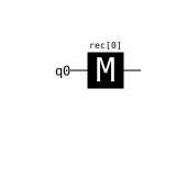
Measurements (M, MX, MY, MZ) project the state into the measurement basis and write the resulting bit into the measurement record.
The measurement record can be used to conditionally apply Pauli gates:
c = Circuit("""M 0CY rec[-1] 1""")c.diagram("timeline-svg", height=170)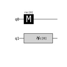
The ! operator can be used to invert the classical measurement bit that is written into the measurement record:
c = Circuit("M !0")c.diagram("timeline-svg", height=120)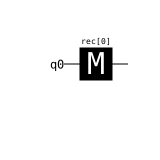
The MPP instruction measures Pauli strings. The MPP can also be used in conjunction with the ! operator to flip the classical measurement bit before writing it into the measurement record.
c = Circuit("MPP !Z0*X2*Y3")c.diagram("timeline-svg", height=260)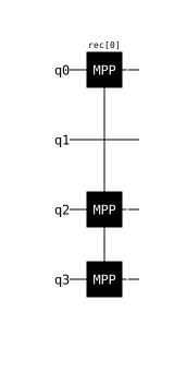
The MXX, MYY, and MZZ instructions measure two-qubit Pauli parity. For example, MZZ measures whether pairs of qubits are in the same-parity subspace () or opposite-parity subspace ().
c = Circuit("MZZ 0 1")c.diagram("timeline-svg", height=170)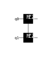
The MPAD instruction pads the measurement record with fixed bit values (0 or 1), without performing any actual measurement.
c = Circuit("MPAD 0 1 1 0")c.diagram("timeline-svg", height=170)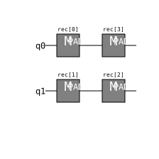
The SPP instruction applies (up to global phase) for a Pauli product , which is equivalent to phasing the eigenspace of by . For example, SPP Z0 is equivalent to the S gate, and SPP X0*X1 is equivalent to SQRT_XX. The SPP_DAG instruction applies (phases by ) instead. The ! operator inverts the product, swapping SPP and SPP_DAG behavior.
c = Circuit("SPP X0*Y1*Z2")c.diagram("timeline-svg", height=220)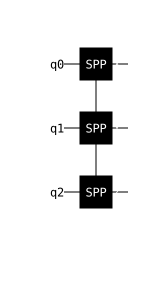
Similarly, TPP applies (up to global phase), phasing the eigenspace by . TPP_DAG applies (phases by ).
c = Circuit(""" SPP Z0 * Z3 * Y4 # TPP X0*Y1 TPP Z0 SPP Z0*Z0*Z1*Z1 TPP_DAG X0*Y1*Z2""")c.diagram("timeline-svg", height=420)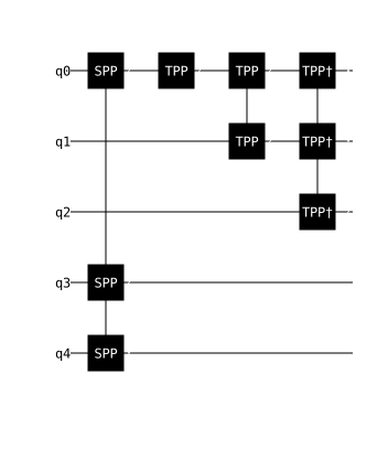
Noise Channels
Tsim supports all noise channels supported by Stim.
The X_ERROR(p) instruction is a X instruction that is applied with probability p.
c = Circuit("X_ERROR(0.1) 0")c.diagram("timeline-svg", height=120)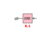
The PAULI_CHANNEL_1(p_x, p_y, p_z) instruction is a X, Y, and Z instruction that is applied with probabilities p_x, p_y, and p_z respectively.
c = Circuit("PAULI_CHANNEL_1(0.1, 0.2, 0.3) 0")c.diagram("timeline-svg", height=120)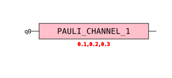
The PAULI_CHANNEL_2 instruction takes fifteen floats specifying the disjoint probabilities of each possible Pauli pair
that can occur (except for the non-error double identity case).
The disjoint probability arguments are (in order):
p_ix, p_iy, p_iz, p_xi, p_xx, p_xy, p_xz, p_yi, p_yx, p_yy, p_yz, p_zi, p_zx, p_zy, p_zz
c = Circuit( "PAULI_CHANNEL_2(0.01, 0.01, 0.03, 0.01, 0.01, 0.01, 0.01, 0.01, 0.01, 0.01, 0.01, 0.01, 0.01, 0.01, 0.01) 0 1")c.diagram("timeline-svg", height=170)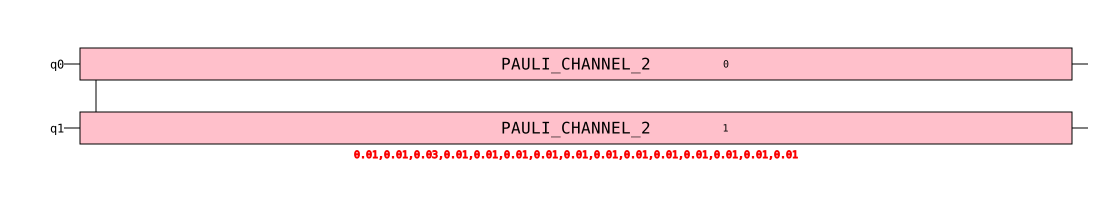
The DEPOLARIZE1(p) instruction applies a randomly chosen Pauli with probability p.
c = Circuit("DEPOLARIZE1(0.01) 0")c.diagram("timeline-svg", height=120)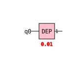
The DEPOLARIZE2(p) instruction applies a randomly chosen two-qubit Pauli with probability p.
c = Circuit("DEPOLARIZE2(0.01) 0 1")c.diagram("timeline-svg", height=170)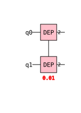
The CORRELATED_ERROR(p) instruction applies a specified Pauli product with probability p. If no error occurred, then a following ELSE_CORRELATED_ERROR(p2) instruction may apply a Pauli product with probabiliy p2. If no error occurs again, further ELSE_CORRELATED_ERROR(pi) instructions in the chain may apply a Pauli products.
c = Circuit("""CORRELATED_ERROR(0.1) X0 # Apply X with probability 0.1ELSE_CORRELATED_ERROR(0.2) Z0 Y1 # If no error occurred, apply Z0*Y1 with probability 0.2ELSE_CORRELATED_ERROR(0.3) X1 # If still no error, apply X1 with probability 0.3""")c.diagram("timeline-svg", height=170)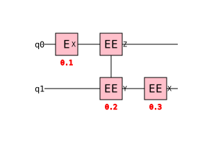
Annotations
Tsim supports detector and observable annotations.
The DETECTOR instruction is only used in detector sampling mode and ignored otherwise. It instructs the detector sampler to record the XOR of classical outcomes of specified measurement bits.
c = Circuit(""" M 0 0 DETECTOR rec[-1] rec[-2]""")c.diagram("timeline-svg", height=150)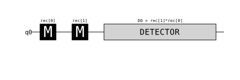
The OBSERVABLE_INCLUDE instruction is only used in observable sampling mode and ignored otherwise. It instructs the detector sampler to record the XOR of the specified measurement bits.
c = Circuit(""" M 0 0 OBSERVABLE_INCLUDE(0) rec[-1] rec[-2]""")c.diagram("timeline-svg", height=150)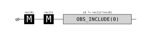
Sampling
Tsim supports multiple samplers. The first is a measurement sampler. This will simply sample bits for each measurement instruction in the circuit. Detector and observable annotations will simply be ignored by this sampler.
c = Circuit(""" RX 0 R 1 CNOT 0 1 M 0 1""")sampler = c.compile_sampler()c.diagram("timeline-svg", height=170)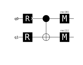
sampler.sample(shots=5)array([[ True, True], [ True, True], [ True, True], [False, False], [ True, True]])The second sampling mode is detector sampling. This will sample detector events and observable values. Detector and observable bits can always be obtained by linear transformations of the measurement bits as return by the measurement sampler. In practice, however, it can be much more efficient to sample detector events directly.
c = Circuit(""" RX 0 R 1 CNOT 0 1 M 0 1 DETECTOR rec[-1] rec[-2] OBSERVABLE_INCLUDE(0) rec[-1]""")sampler = c.compile_detector_sampler()c.diagram("timeline-svg", height=170)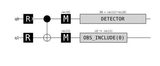
detectors, observables = sampler.sample(5, separate_observables=True)print(detectors)print(observables)[[False] [False] [False] [False] [False]][[False] [False] [ True] [False] [False]]Finally, Tsim allows to compute probability values for target states via the CompiledStateProbs sampler.
import numpy as npfrom tsim.sampler import CompiledStateProbs
sampler = CompiledStateProbs(c)sampler.probability_of(np.array([0, 0]), batch_size=1)array([0.5], dtype=float32)sampler.probability_of(np.array([0, 1]), batch_size=1)array([0.], dtype=float32)sampler.probability_of(np.array([1, 0]), batch_size=1)array([0.], dtype=float32)sampler.probability_of(np.array([1, 1]), batch_size=1)array([0.5], dtype=float32)Visualization
Tsim supports multiple ways of visualizing quantum circuits.
The timeline-svg diagram shows the circuit as a time-ordered sequence of gates.
c = Circuit(""" QUBIT_COORDS(0, 0) 0 # specifies qubit coordinates for the "timeslice-svg" diagram QUBIT_COORDS(1, 1) 1 H 0 TICK T 0 H 0 TICK CNOT 0 1 TICK DEPOLARIZE2(0.1) 0 1 TICK R_Z(0.2) 1 TICK M 0 1 DETECTOR rec[-1] rec[-2] OBSERVABLE_INCLUDE(0) rec[-1]""")c.diagram("timeline-svg", height=170)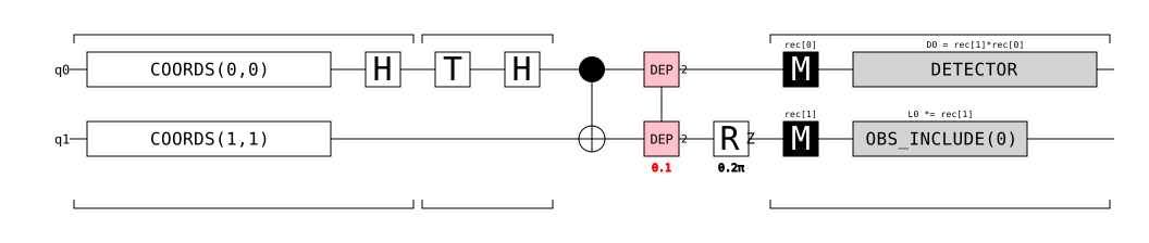
When TICK instructions are present, each tick can be shown as a 2D time slice with the timeslice-svg diagram. Here, QUBIT_COORDS annotations can be used to specify the 2D coordinates of the qubits.
c.diagram("timeslice-svg", width=800, rows=1)
With the pyzx argument, the circuit can be visualized using the pyzx as a ZX-diagram.
c.diagram("pyzx");The pyzx-meas and pyzx-dets diagrams show ZX diagrams where outputs represent probabilities of measurement outcomes for measurement and detector/observables, respectively.
c.diagram("pyzx-meas", scale_horizontally=2);c.diagram("pyzx-dets", scale_horizontally=1.5);Detector Error Models
Tsim allows to compute detector error models from a circuit. The method Circuit.detector_error_model() computes a stim.DetectorErrorModel from the circuit. As opposed to Stim, detectors and observables need not be deterministic.
c = Circuit(""" RX 0 R 1 CNOT 0 1 DEPOLARIZE1(0.1) 0 1 M 0 1 DETECTOR rec[-1] rec[-2] DETECTOR rec[-1]""")c.detector_error_model()stim.DetectorErrorModel(''' error(0.0666667) D0 error(0.0666667) D0 D1 error(0.5) D1''')